Project 3 - News Popularity Data
Link to my rendered project Readme file : here
The above file has the link to each document created for this project.
Link to my project 3 repository : here
Overview
I finished my third project for the ST558: Data Science for Statisticians course that revolved around doing some exploratory Data Analysis and modelling for a data set on news articles. The target variable for this project was the number of shares each type of news article had. The types of articles that are dealt with in this project are:
- Technology
- Lifestyle
- Entertainment
- Business
- Social Media
- World
Initially the data set containing details about all these articles is taken in consideration, and using the params function feature in YML header in R markdown, the data set related just with one particular type of article is fetched, and is repeated for all types of articles. The Render function included in the Readme files depicts how that is achieved.
Some new variables were also created from the existing variables in the data set to understand a trend in the data, for example, the title sentiment polarity was created as a classifaiction variable to catergorize any given title into either positive sentiment or negative sentimment bucket.
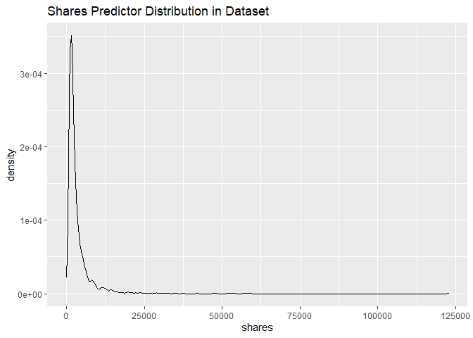
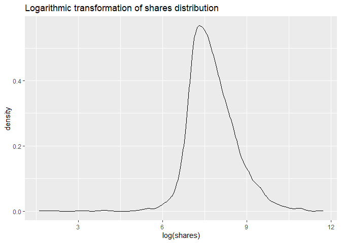
We were interested in predicting the number of shares for each article, hence we had to make sure that the response variable had a proper distribution. Up on doing inital exploratory data analysis, it was found that the number of shares in the data was skewed, and hence to remedy that, we took the logarithmic transformation of the response variable, and built all our models using that variable as the reponse variable.


Linear Models
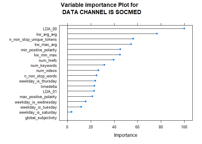
Since we were dealing with prediction of shares for each type of articles, we needed a set of predicting variables for the modelling. This data set had a huge dimensionality, and hence proper variable selection and substituion became imminent. We initially ran a linear regression model that had all the available variables, and found the statistically significant variables from that, and automated the technique to use those variables in subsequent linear models. The most statistically significant variables were then used to build a simple multiple linear regression model.
After the linear regression model, a LASSO model was built that provides an improvement over the linear regression model in cases with less number of variables. This became true when we used only the statistically significant variables from the first step. The statistics included in the project depicts that the LASSO model overall proved to be a good improvement over the linear regression model.

Ensemble Models
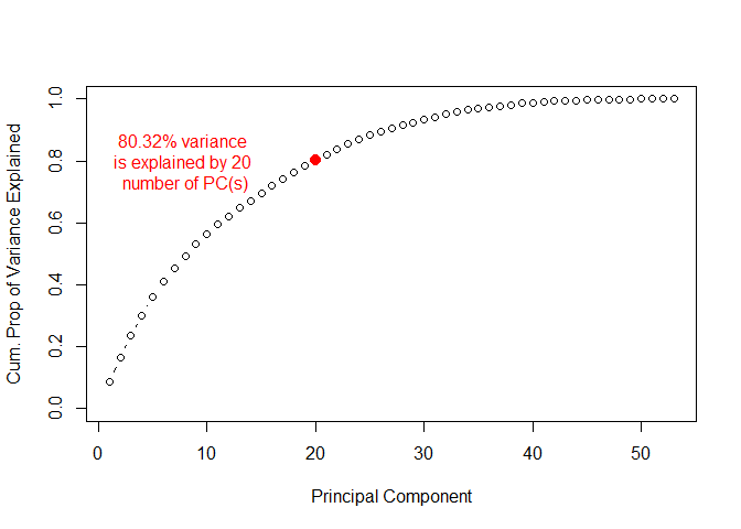
After fitting LASSO model, we then moved to the ensemble learning methods. The first model built was the Random Forest model. Moving to the ensemble learning method, we decided to try a new approach for best variable selection. Before fitting any models, we decided to create Principle Components from all the variables in the data set, and use the first n number of PCs that explained a good enough variance in the data set (at least 80%). We then used the created PCs to fit a random forest model with log shares as the target variable, and mtry as the tuning parameter. In some cases this model performed better than previous models, in cases not.

The last model that we built was the Boosted Tree model. In this, we used all the available variables to create the model. Since boosted tree works on slow learning of the trees from the best variables, we decided to let the model select its variables. We also used tuned several hyperparameters to select a “best” model.
Comparing All Models
Since almost all the models that we had cretaed had different number of independent variables, we couldn’t really use the R2 value of the model as a comparison metric, hence we calculated the Adjusted R2 value for each model, and added that in the model comparison table shown in the project file. A best model from linear models, a best model from ensemble models, and a best overall models were selected from their prediction RMSE values. In case the RMSE values were same, we used the Adjusted R2 values to take a decision; the higher the adjusted R2 value, better the model.
Conclusion
All of these steps mentioned above, from selecting best variables for the model, till selecting best model, are all automated in the project. The process is repeated for each type of articles that we are dealing with, and in the end, we get 6 files as an output, to which link has been provided in the project Readme file.
What would I do differently?
If there wasn’t any computational constarint, I would have further selected more or a broader range of hyperparamters for tuning the model. For the case of linear models, I would extend my range to Ridge regression as well, to see how that compares with the current models. I would also use the created PCs in the data to fit some other regression models as well, to also compare them with the current ones. I would also check if taking transformations of the independent variables could help improvise any models.
The most difficult part
One of the challenging parts of the project was the realization of presence of skewness in the data. Once we had a clarity of skweness, we then tried taking a few trial and error transformations for the shares variable, and then finalized the log transformation works best to make the data normally distributed. Another challenge was to select the best variables from the data set, automating the statistically significant variables, and selecting the PCs was a good challenge as well.
Takeaways
- Always plot the target variable first, and then decide on model selection
- Select the tune parameter range wisely, in order to minimize computational force
- Initial EDA goes a long way, helps in seeing patterns, and selecting some important variables for the model
- Feature modelling is as important as regression modelling